PyTorch Introduction

TA: Chi-Liang Liu

This Tutorial is modified from University of Washington CSE446 and PyTorch Official Tutorials

Today, we will be intoducing PyTorch, "an open source deep learning platform that provides a seamless path from research prototyping to production deployment".

This notebook is by no means comprehensive. If you have any questions the documentation and Google are your friends.

Goal takeaways:

• Automatic differentiation is a powerful tool
• PyTorch implements common functions used in deep learning
• Data Processing with PyTorch DataSet
• Mixed Presision Training in PyTorch

Tensors and relation to numpy

By this point, we have worked with numpy quite a bit. PyTorch's basic building block, the tensor is similar to numpy's ndarray

# we create tensors in a similar way to numpy nd arrays
x_numpy = np.array([0.1, 0.2, 0.3])
x_torch = torch.tensor([0.1, 0.2, 0.3])
print('x_numpy, x_torch')
print(x_numpy, x_torch)
print()

# to and from numpy, pytorch
print('to and from numpy and pytorch')
print(torch.from_numpy(x_numpy), x_torch.numpy())
print()

# we can do basic operations like +-*/
y_numpy = np.array([3,4,5.])
y_torch = torch.tensor([3,4,5.])
print("x+y")
print(x_numpy + y_numpy, x_torch + y_torch)
print()

# many functions that are in numpy are also in pytorch
print("norm")
print(np.linalg.norm(x_numpy), torch.norm(x_torch))
print()

# to apply an operation along a dimension,
# we use the dim keyword argument instead of axis
print("mean along the 0th dimension")
x_numpy = np.array([[1,2],[3,4.]])
x_torch = torch.tensor([[1,2],[3,4.]])
print(np.mean(x_numpy, axis=0), torch.mean(x_torch, dim=0))

Tensor.view

We can use the Tensor.view() function to reshape tensors similarly to numpy.reshape()

It can also automatically calculate the correct dimension if a -1 is passed in. This is useful if we are working with batches, but the batch size is unknown.

# "MNIST"
N, C, W, H = 10000, 3, 28, 28
X = torch.randn((N, C, W, H))

print(X.shape)
print(X.view(N, C, 784).shape)
print(X.view(-1, C, 784).shape) # automatically choose the 0th dimension

Computation graphs

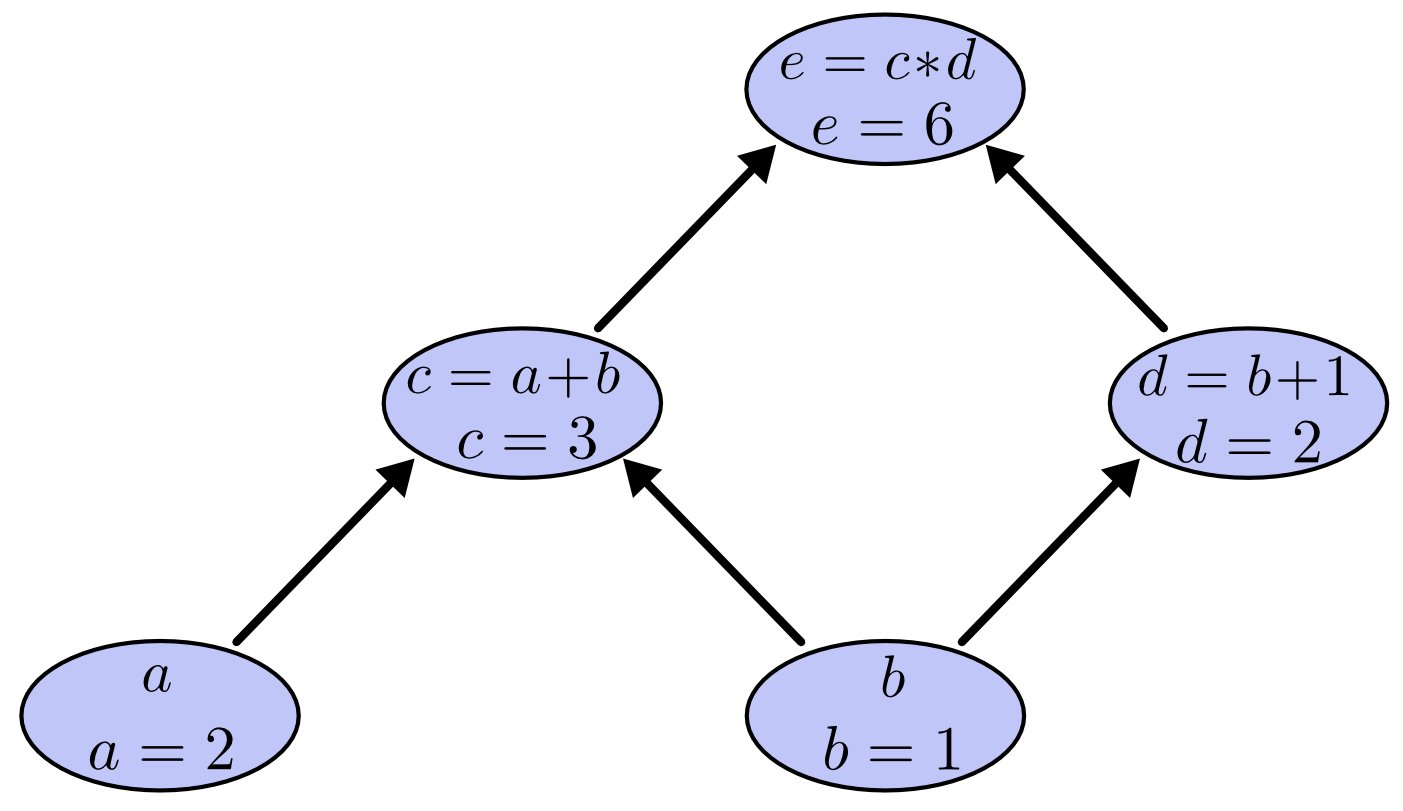
What's special about PyTorch's tensor object is that it implicitly creates a computation graph in the background. A computation graph is a a way of writing a mathematical expression as a graph. There is an algorithm to compute the gradients of all the variables of a computation graph in time on the same order it is to compute the function itself.

Consider the expression $e=(a+b)*(b+1)$ with values $a=2, b=1$. We can draw the evaluated computation graph as

In PyTorch, we can write this as

source

a = torch.tensor(2.0, requires_grad=True) # we set requires_grad=True to let PyTorch know to keep the graph
b = torch.tensor(1.0, requires_grad=True)
c = a + b
d = b + 1
e = c * d
print('c', c)
print('d', d)
print('e', e)

We can see that PyTorch kept track of the computation graph for us.

PyTorch as an auto grad framework

Now that we have seen that PyTorch keeps the graph around for us, let's use it to compute some gradients for us.

Consider the function $f(x) = (x-2)^2$.

Q: Compute $\frac{d}{dx} f(x)$ and then compute $f'(1)$.

We make a backward() call on the leaf variable (y) in the computation, computing all the gradients of y at once.

def f(x):
    return (x-2)**2

def fp(x):
    return 2*(x-2)

x = torch.tensor([1.0], requires_grad=True)

y = f(x)
y.backward()

print('Analytical f\'(x):', fp(x))
print('PyTorch\'s f\'(x):', x.grad)

It can also find gradients of functions.

Let $w = [w_1, w_2]^T$

Consider $g(w) = 2w_1w_2 + w_2\cos(w_1)$

Q: Compute $\nabla_w g(w)$ and verify $\nabla_w g([\pi,1]) = [2, \pi - 1]^T$

def g(w):
    return 2*w[0]*w[1] + w[1]*torch.cos(w[0])

def grad_g(w):
    return torch.tensor([2*w[1] - w[1]*torch.sin(w[0]), 2*w[0] + torch.cos(w[0])])

w = torch.tensor([np.pi, 1], requires_grad=True)

z = g(w)
z.backward()

print('Analytical grad g(w)', grad_g(w))
print('PyTorch\'s grad g(w)', w.grad)

Using the gradients

Now that we have gradients, we can use our favorite optimization algorithm: gradient descent!

Let $f$ the same function we defined above.

Q: What is the value of $x$ that minimizes $f$?

x = torch.tensor([5.0], requires_grad=True)
step_size = 0.25

print('iter,\tx,\tf(x),\tf\'(x),\tf\'(x) pytorch')
for i in range(15):
    y = f(x)
    y.backward() # compute the gradient
    
    print('{},\t{:.3f},\t{:.3f},\t{:.3f},\t{:.3f}'.format(i, x.item(), f(x).item(), fp(x).item(), x.grad.item()))
    
    x.data = x.data - step_size * x.grad # perform a GD update step
    
    # We need to zero the grad variable since the backward()
    # call accumulates the gradients in .grad instead of overwriting.
    # The detach_() is for efficiency. You do not need to worry too much about it.
    x.grad.detach_()
    x.grad.zero_()

Linear Regression

Now, instead of minimizing a made-up function, lets minimize a loss function on some made-up data.

We will implement Gradient Descent in order to solve the task of linear regression.

# make a simple linear dataset with some noise

d = 2
n = 50
X = torch.randn(n,d)
true_w = torch.tensor([[-1.0], [2.0]])
y = X @ true_w + torch.randn(n,1) * 0.1
print('X shape', X.shape)
print('y shape', y.shape)
print('w shape', true_w.shape)

Sanity check

To verify PyTorch is computing the gradients correctly, let's recall the gradient for the RSS objective:

$$\nabla_w \mathcal{L}_{RSS}(w; X) = \nabla_w\frac{1}{n} ||y - Xw||_2^2 = -\frac{2}{n}X^T(y-Xw)$$

# define a linear model with no bias
def model(X, w):
    return X @ w

# the residual sum of squares loss function
def rss(y, y_hat):
    return torch.norm(y - y_hat)**2 / n

# analytical expression for the gradient
def grad_rss(X, y, w):
    return -2*X.t() @ (y - X @ w) / n

w = torch.tensor([[1.], [0]], requires_grad=True)
y_hat = model(X, w)

loss = rss(y, y_hat)
loss.backward()

print('Analytical gradient', grad_rss(X, y, w).detach().view(2).numpy())
print('PyTorch\'s gradient', w.grad.view(2).numpy())

Now that we've seen PyTorch is doing the right think, let's use the gradients!

Linear regression using GD with automatically computed derivatives

We will now use the gradients to run the gradient descent algorithm.

Note: This example is an illustration to connect ideas we have seen before to PyTorch's way of doing things. We will see how to do this in the "PyTorchic" way in the next example.

step_size = 0.1

print('iter,\tloss,\tw')
for i in range(20):
    y_hat = model(X, w)
    loss = rss(y, y_hat)
    
    loss.backward() # compute the gradient of the loss
    
    w.data = w.data - step_size * w.grad # do a gradient descent step
    
    print('{},\t{:.2f},\t{}'.format(i, loss.item(), w.view(2).detach().numpy()))
    
    # We need to zero the grad variable since the backward()
    # call accumulates the gradients in .grad instead of overwriting.
    # The detach_() is for efficiency. You do not need to worry too much about it.
    w.grad.detach()
    w.grad.zero_()

print('\ntrue w\t\t', true_w.view(2).numpy())
print('estimated w\t', w.view(2).detach().numpy())

torch.nn.Module

Module is PyTorch's way of performing operations on tensors. Modules are implemented as subclasses of the torch.nn.Module class. All modules are callable and can be composed together to create complex functions.

torch.nn docs

Note: most of the functionality implemented for modules can be accessed in a functional form via torch.nn.functional, but these require you to create and manage the weight tensors yourself.

torch.nn.functional docs.

Linear Module

The bread and butter of modules is the Linear module which does a linear transformation with a bias. It takes the input and output dimensions as parameters, and creates the weights in the object.

Unlike how we initialized our $w$ manually, the Linear module automatically initializes the weights randomly. For minimizing non convex loss functions (e.g. training neural networks), initialization is important and can affect results. If training isn't working as well as expected, one thing to try is manually initializing the weights to something different from the default. PyTorch implements some common initializations in torch.nn.init.

torch.nn.init docs

d_in = 3
d_out = 4
linear_module = nn.Linear(d_in, d_out)

example_tensor = torch.tensor([[1.,2,3], [4,5,6]])
# applys a linear transformation to the data
transformed = linear_module(example_tensor)
print('example_tensor', example_tensor.shape)
print('transormed', transformed.shape)
print()
print('We can see that the weights exist in the background\n')
print('W:', linear_module.weight)
print('b:', linear_module.bias)

Activation functions

PyTorch implements a number of activation functions including but not limited to ReLU, Tanh, and Sigmoid. Since they are modules, they need to be instantiated.

activation_fn = nn.ReLU() # we instantiate an instance of the ReLU module
example_tensor = torch.tensor([-1.0, 1.0, 0.0])
activated = activation_fn(example_tensor)
print('example_tensor', example_tensor)
print('activated', activated)

Sequential

Many times, we want to compose Modules together. torch.nn.Sequential provides a good interface for composing simple modules.

d_in = 3
d_hidden = 4
d_out = 1
model = torch.nn.Sequential(
                            nn.Linear(d_in, d_hidden),
                            nn.Tanh(),
                            nn.Linear(d_hidden, d_out),
                            nn.Sigmoid()
                           )

example_tensor = torch.tensor([[1.,2,3],[4,5,6]])
transformed = model(example_tensor)
print('transformed', transformed.shape)

Note: we can access all of the parameters (of any nn.Module) with the parameters() method.

params = model.parameters()

for param in params:
    print(param)

Loss functions

PyTorch implements many common loss functions including MSELoss and CrossEntropyLoss.

mse_loss_fn = nn.MSELoss()

input = torch.tensor([[0., 0, 0]])
target = torch.tensor([[1., 0, -1]])

loss = mse_loss_fn(input, target)

print(loss)

torch.optim

PyTorch implements a number of gradient-based optimization methods in torch.optim, including Gradient Descent. At the minimum, it takes in the model parameters and a learning rate.

Optimizers do not compute the gradients for you, so you must call backward() yourself. You also must call the optim.zero_grad() function before calling backward() since by default PyTorch does and inplace add to the .grad member variable rather than overwriting it.

This does both the detach_() and zero_() calls on all tensor's grad variables.

torch.optim docs

# create a simple model
model = nn.Linear(1, 1)

# create a simple dataset
X_simple = torch.tensor([[1.]])
y_simple = torch.tensor([[2.]])

# create our optimizer
optim = torch.optim.SGD(model.parameters(), lr=1e-2)
mse_loss_fn = nn.MSELoss()

y_hat = model(X_simple)
print('model params before:', model.weight)
loss = mse_loss_fn(y_hat, y_simple)
optim.zero_grad()
loss.backward()
optim.step()
print('model params after:', model.weight)

As we can see, the parameter was updated in the correct direction

Linear regression using GD with automatically computed derivatives and PyTorch's Modules

Now let's combine what we've learned to solve linear regression in a "PyTorchic" way.

step_size = 0.1

linear_module = nn.Linear(d, 1, bias=False)

loss_func = nn.MSELoss()

optim = torch.optim.SGD(linear_module.parameters(), lr=step_size)

print('iter,\tloss,\tw')

for i in range(20):
    y_hat = linear_module(X)
    loss = loss_func(y_hat, y)
    optim.zero_grad()
    loss.backward()
    optim.step()
    
    print('{},\t{:.2f},\t{}'.format(i, loss.item(), linear_module.weight.view(2).detach().numpy()))

print('\ntrue w\t\t', true_w.view(2).numpy())
print('estimated w\t', linear_module.weight.view(2).detach().numpy())

Linear regression using SGD

In the previous examples, we computed the average gradient over the entire dataset (Gradient Descent). We can implement Stochastic Gradient Descent with a simple modification.

step_size = 0.01

linear_module = nn.Linear(d, 1)
loss_func = nn.MSELoss()
optim = torch.optim.SGD(linear_module.parameters(), lr=step_size)
print('iter,\tloss,\tw')
for i in range(200):
    rand_idx = np.random.choice(n) # take a random point from the dataset
    x = X[rand_idx] 
    y_hat = linear_module(x)
    loss = loss_func(y_hat, y[rand_idx]) # only compute the loss on the single point
    optim.zero_grad()
    loss.backward()
    optim.step()
    
    if i % 20 == 0:
        print('{},\t{:.2f},\t{}'.format(i, loss.item(), linear_module.weight.view(2).detach().numpy()))

print('\ntrue w\t\t', true_w.view(2).numpy())
print('estimated w\t', linear_module.weight.view(2).detach().numpy())

CrossEntropyLoss

So far, we have been considering regression tasks and have used the MSELoss module. For the homework, we will be performing a classification task and will use the cross entropy loss.

PyTorch implements a version of the cross entropy loss in one module called CrossEntropyLoss. Its usage is slightly different than MSE, so we will break it down here.

• input: The first parameter to CrossEntropyLoss is the output of our network. It expects a real valued tensor of dimensions $(N,C)$ where $N$ is the minibatch size and $C$ is the number of classes. In our case $N=3$ and $C=2$. The values along the second dimension correspond to raw unnormalized scores for each class. The CrossEntropyLoss module does the softmax calculation for us, so we do not need to apply our own softmax to the output of our neural network.
• output: The second parameter to CrossEntropyLoss is the true label. It expects an integer valued tensor of dimension $(N)$. The integer at each element corresponds to the correct class. In our case, the "correct" class labels are class 0, class 1, and class 1.

Try out the loss function on three toy predictions. The true class labels are $y=[1,1,0]$. The first two examples correspond to predictions that are "correct" in that they have higher raw scores for the correct class. The second example is "more confident" in the prediction, leading to a smaller loss. The last two examples are incorrect predictions with lower and higher confidence respectively.

loss = nn.CrossEntropyLoss()

input = torch.tensor([[-1., 1],[-1, 1],[1, -1]]) # raw scores correspond to the correct class
# input = torch.tensor([[-3., 3],[-3, 3],[3, -3]]) # raw scores correspond to the correct class with higher confidence
# input = torch.tensor([[1., -1],[1, -1],[-1, 1]]) # raw scores correspond to the incorrect class
# input = torch.tensor([[3., -3],[3, -3],[-3, 3]]) # raw scores correspond to the incorrect class with incorrectly placed confidence

target = torch.tensor([1, 1, 0])
output = loss(input, target)
print(output)

Learning rate schedulers

Often we do not want to use a fixed learning rate throughout all training. PyTorch offers learning rate schedulers to change the learning rate over time. Common strategies include multiplying the lr by a constant every epoch (e.g. 0.9) and halving the learning rate when the training loss flattens out.

See the learning rate scheduler docs for usage and examples

Convolutions

When working with images, we often want to use convolutions to extract features using convolutions. PyTorch implments this for us in the torch.nn.Conv2d module. It expects the input to have a specific dimension $(N, C_{in}, H_{in}, W_{in})$ where $N$ is batch size, $C_{in}$ is the number of channels the image has, and $H_{in}, W_{in}$ are the image height and width respectively.

We can modify the convolution to have different properties with the parameters:

• kernel_size
• stride
• padding

They can change the output dimension so be careful.

See the torch.nn.Conv2d docs for more information.

To illustrate what the Conv2d module is doing, let's set the conv weights manually to a Gaussian blur kernel.

We can see that it applies the kernel to the image.

# a gaussian blur kernel
gaussian_kernel = torch.tensor([[1., 2, 1],[2, 4, 2],[1, 2, 1]]) / 16.0

conv = nn.Conv2d(1, 1, 3)
# manually set the conv weight
conv.weight.data[:] = gaussian_kernel

convolved = conv(image_torch)

plt.title('original image')
plt.imshow(image_torch.view(28,28).detach().numpy())
plt.show()

plt.title('blurred image')
plt.imshow(convolved.view(26,26).detach().numpy())
plt.show()

As we can see, the image is blurred as expected.

In practice, we learn many kernels at a time. In this example, we take in an RGB image (3 channels) and output a 16 channel image. After an activation function, that could be used as input to another Conv2d module.

im_channels = 3 # if we are working with RGB images, there are 3 input channels, with black and white, 1
out_channels = 16 # this is a hyperparameter we can tune
kernel_size = 3 # this is another hyperparameter we can tune
batch_size = 4
image_width = 32
image_height = 32

im = torch.randn(batch_size, im_channels, image_width, image_height)

m = nn.Conv2d(im_channels, out_channels, kernel_size)
convolved = m(im) # it is a module so we can call it

print('im shape', im.shape)
print('convolved im shape', convolved.shape)

Useful links:

• 60 minute PyTorch Tutorial
• PyTorch Docs
• Lecture notes on Auto-Diff

Custom Datasets, DataLoaders

This is modified from pytorch official tutorial. Author: Sasank Chilamkurthy <https://chsasank.github.io>_

A lot of effort in solving any machine learning problem goes in to preparing the data. PyTorch provides many tools to make data loading easy and hopefully, to make your code more readable. In this tutorial, we will see how to load and preprocess/augment data from a non trivial dataset.

Dataset class

torch.utils.data.Dataset is an abstract class representing a dataset. Your custom dataset should inherit Dataset and override the following methods:

• __len__ so that len(dataset) returns the size of the dataset.
• __getitem__ to support the indexing such that dataset[i] can be used to get $i$\ th sample

Let's create a dataset class for our face landmarks dataset. We will read the csv in __init__ but leave the reading of images to __getitem__. This is memory efficient because all the images are not stored in the memory at once but read as required.

Sample of our dataset will be a dict {'image': image, 'landmarks': landmarks}. Our dataset will take an optional argument transform so that any required processing can be applied on the sample. We will see the usefulness of transform in the next section.

class FaceLandmarksDataset(Dataset):
    """Face Landmarks dataset."""

    def __init__(self, csv_file, root_dir, transform=None):
        """
        Args:
            csv_file (string): Path to the csv file with annotations.
            root_dir (string): Directory with all the images.
            transform (callable, optional): Optional transform to be applied
                on a sample.
        """
        self.landmarks_frame = pd.read_csv(csv_file)
        self.root_dir = root_dir
        self.transform = transform

    def __len__(self):
        return len(self.landmarks_frame)

    def __getitem__(self, idx):
        if torch.is_tensor(idx):
            idx = idx.tolist()

        img_name = os.path.join(self.root_dir,
                                self.landmarks_frame.iloc[idx, 0])
        image = io.imread(img_name)
        landmarks = self.landmarks_frame.iloc[idx, 1:]
        landmarks = np.array([landmarks])
        landmarks = landmarks.astype('float').reshape(-1, 2)
        sample = {'image': image, 'landmarks': landmarks}

        if self.transform:
            sample = self.transform(sample)

        return sample

However, we are losing a lot of features by using a simple for loop to iterate over the data. In particular, we are missing out on:

• Batching the data
• Shuffling the data
• Load the data in parallel using multiprocessing workers.

torch.utils.data.DataLoader is an iterator which provides all these features. Parameters used below should be clear. One parameter of interest is collate_fn. You can specify how exactly the samples need to be batched using collate_fn. However, default collate should work fine for most use cases.

dataloader = DataLoader(transformed_dataset, batch_size=4,
                        shuffle=True, num_workers=4)

for i_batch, sample_batched in enumerate(dataloader):
    print(i_batch, sample_batched['image'].size(),
          sample_batched['landmarks'].size())

Mixed Presision Training

Author: Chi-Liang Liu <https://liangtaiwan.github.io> Ref: https://github.com/NVIDIA/apex Using mixed precision to train your networks can be:

• 2-4x faster
• memory-efficient in only 3 lines of Python.

Apex

NVIDIA-maintained utilities to streamline mixed precision and distributed training in Pytorch. Some of the code here will be included in upstream Pytorch eventually. The intention of Apex is to make up-to-date utilities available to users as quickly as possible.

apex.amp

Amp allows users to easily experiment with different pure and mixed precision modes. Commonly-used default modes are chosen by selecting an "optimization level" or opt_level; each opt_level establishes a set of properties that govern Amp's implementation of pure or mixed precision training. Finer-grained control of how a given opt_level behaves can be achieved by passing values for particular properties directly to amp.initialize. These manually specified values override the defaults established by the opt_level.

# Declare model and optimizer as usual, with default (FP32) precision
model = torch.nn.Linear(D_in, D_out).cuda()
optimizer = torch.optim.SGD(model.parameters(), lr=1e-3)

# Allow Amp to perform casts as required by the opt_level
model, optimizer = amp.initialize(model, optimizer, opt_level="O1")
...
# loss.backward() becomes:
with amp.scale_loss(loss, optimizer) as scaled_loss:
    scaled_loss.backward()
...